Designing for feel

Players judge a drive or a compressor less by how accurate it is than by how it responds to them. A drive cleans up when they pick lightly, thickens when they dig in, and blooms or sags over the life of a note. This page is about building that behaviour on purpose and measuring it, rather than hoping it emerges.

Inspiration and listening still choose the final values. What this page offers is a vocabulary. Most of what players call feel comes from a short list of physical mechanisms, and each one can be named, built in Faust and checked with a plot. Classic circuits have these mechanisms as side effects of their parts. A new design can pick the ones it wants, exaggerate them, give them a control or point them somewhere a circuit could not.

The mechanics of adding an effect are in Adding an effect. Where ideas come from is in Designing new sounds.

What a static clipper can't do

Most nonlinear stages here follow one pattern: a fixed filter, a memoryless waveshaper inside pk.oversample4, then another fixed filter. That pattern gets two things right:

• the harmonics depend on input level, through the shape of the curve
• the harmonics depend on frequency, through the filters on either side (BassDrive’s pre-emphasis, MidHump’s clipped feedback branch)

It can’t make anything depend on what was played a moment ago. The first millisecond of a pick attack and the tenth second of the sustain go through the same curve. A lot of what players describe as feel is about time: the tone settling after the attack, a loud chord leaving the next quiet note rougher, a drive that recovers rather than snapping back. All of that needs state that follows the playing.

Mechanisms

Mechanism	What the player notices	How to build it here	How to measure it
Cleanup curve	Picking strength moves the sound from clean to driven, gradually or abruptly	The waveshaper’s knee (kneeClip’s n, softSat’s level) and the gain before it	harmonic_trajectory: harmonics against input level
Level-dependent EQ	Digging in gets brighter, darker or more mid-focused	Filters around the clipper, or a clipped branch summed with a clean one (MidHump)	transfer from noise at several input levels
Bias shift	Hard playing adds even harmonics that build up and fade; at extremes, sputter and gating	pk.biasShift feeding pk.biased(f) in pk.oversample4c	burst and pluck with harmonics_over_time, H2 against time
Sag	Loud passages compress and soften, then recover	A base-rate envelope that lowers the clip level, passed in with oversample4c	Output level and THD against time on a burst
Attack against sustain	Transients and tails are treated differently	An envelope or transient detector that drives a control	pluck with harmonics_over_time, attack against tail
Blocking and recovery	After an overload the stage goes thin or quiet, then comes back	A large biasShift with a slow release, or sag with a long recovery	burst: fundamental level after the loud section
Program-dependent timing	A compressor releases faster after a short peak than after a long passage	Two envelopes with different time constants, combined	Gain against time after bursts of different lengths
Interacting controls	One knob moves several things along a path chosen by ear	Map one control to several constants	Whatever the moved constants affect, at several knob positions

These mechanisms come from analyses of real circuits. Bias shift and blocking distortion in valve stages are described in Blencowe [3]. Yeh [1] and Pakarinen and Yeh [2] cover simulation of distortion circuits and why static waveshapers miss behaviour that changes with level and time.

Building state into a nonlinearity

pk.oversample4(f) applies f to four phase streams in parallel, so f must have no memory. The way round that is to split the stage in two:

1. A base-rate control path with all the memory: an envelope follower, a charging capacitor, a slow detector. It produces a smooth control signal c.
2. A memoryless shaper f(x, c) that takes the control as a second input. It runs inside pk.oversample4c(f), which holds c for the four phases of each sample and lines it up with the interpolated audio.

// f(x, b): the shaper, moved off centre by b
clip  = pk.biased(pk.softSat(0.6));
// base rate: charges on peaks, recovers slowly
bias  = pk.biasShift(0.6, 0.3, 0.015, 0.15);
stage = _ <: _, bias : pk.oversample4c(clip);

A sag stage follows the same pattern, with the control as a headroom that scales the clip level:

// h = 1 at rest, smaller when loud
sagged(f, x, h) = h * f(x / h);
headroom = an.amp_follower_ar(0.005, 0.3)
         : \(e).(1 / (1 + 0.5 * e));
stage = _ <: _, headroom : pk.oversample4c(sagged(pk.softSat(0.6)));

Rules for the control path:

• Keep it smooth. c is held across the four phases, which is only valid if it has little energy near the base Nyquist frequency. Envelopes with time constants of a few milliseconds or more are fine. Check the aliasing against render_1x with the control at its most active, as tests/midhump/test_dynamics.py does.
• Shape first, then smooth. If the control saturates, saturate the target before the smoother. Otherwise a hard-driven input reaches the limit on its first cycle, and the time constants stop meaning anything. pk.biasShift is built this way.
• Derive it from the signal before the shaper. A feed-forward control has no loop delay. Taking it from the oversampler’s output puts its 32-sample latency inside the loop, which is fine for time constants of tens of milliseconds and wrong for anything faster.
• Make zero mean off. At its minimum setting a new control should give the same output as the effect without it. pk.biased(f)(x, 0) is f(x), so MidHump’s Bloom at 0 is the published circuit. Measured against the build before Bloom was added, the largest difference is 8 × 10⁻⁷ (about −122 dBFS), which is float rounding.

Clipping inside a feedback loop at audio rate (an op-amp whose clipped output feeds back through a frequency-dependent network) can’t be split this way. It needs the loop solved at the oversampled rate, which pedalkit.lib doesn’t support yet.

Measuring feel

The standard tests are steady state. Behaviour over time and level needs four more helpers from tests/lib/fxtest.py (see Tests and measurements):

Helper	Signal	What it shows
harmonic_trajectory(f0, levels_db)	Steady sines at a range of levels	The cleanup curve: where each harmonic appears and how it grows
burst(f0, [quiet, loud, quiet], durs)	A tone that steps down after a loud passage	Memory: what a loud passage leaves behind, and how long it lasts
pluck(f0, dur, decay=...)	A sharp attack with an exponential decay	Attack against sustain over one note. Use n=1 to measure the harmonics the effect adds.
harmonics_over_time(y, f0)	Any of the above, analysed in short windows	DC and each harmonic against time

Put the behaviour you want in the design notes as numbers, so the tests can check it. For example:

• THD rises from 1 % to 10 % over at least 18 dB of input (a gradual cleanup curve)
• H2 builds up between 10 ms and 100 ms after a loud onset, and is gone 1 s after the playing gets quiet
• the output of a sustained 0 dBFS tone drops by 3 dB over 200 ms and recovers within 500 ms (sag)
• below −40 dBFS input the new control changes nothing

harmonics_over_time uses a window of a whole number of periods (four by default), so a steady tone reads without leakage between harmonics. Windows that straddle a step in level read the step itself as harmonics. Skip them when you time a rise, as test_dynamics.py does.

Worked example: MidHump’s Bloom

MidHump’s clipping diodes sit in an op-amp’s feedback path, where nothing can bias them, so the pedal’s clipping is symmetric and the same on every cycle. The Bloom control gives the diodes a bias that charges up on loud peaks and drains away afterwards. The constants and their intent are in the design notes.

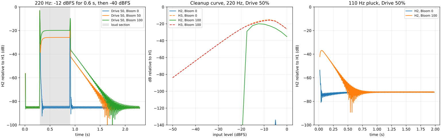
Data: dynamics.csv.

• Left: at Bloom 0 the second harmonic stays at the analysis floor. At Bloom 100 it settles at −20 dBc on a loud tone, and after the loud section it decays over about a second.
• Middle: H2 appears only above the diode knee. H3 doesn’t change, so quiet playing and the odd-order character are left alone.
• Right: on a plucked note, H2 peaks about 50 ms in, after the first cycles, and decays with the note.

All of this is checked in tests/midhump/test_dynamics.py. Whether it sounds like the drive answering the hand is the open question in the design notes, and only listening can settle it.

What to listen for

Measurement narrows the search, but the last step is a person playing. Give whoever listens a fixed set of checks, and tie each one to the constant it would change:

Check	Listen for	Usually set by
Soft against hard picking	A smooth path from clean to driven, with no step	The knee and the gain before it
Guitar volume rolled back	The effect cleaning up instead of only getting quieter	The knee, and any threshold on a dynamic control
Palm mutes and fast riffs	Notes staying distinct; no smearing or pumping	Attack and release times
Chords	Clarity against mush; intermodulation	Clip hardness, pre-filtering, the amount of bias shift
Single notes held	How the tone changes as the note decays, and whether that is a swell or a collapse	Release times, the size of the shift or sag
After a loud passage	Whether the quiet notes after it carry a welcome roughness or sound broken	Release times

Record what was heard and at which settings in the effect’s design notes, under open questions, or in an issue with the needs-listening label.

Sources

1. D. T. Yeh, Digital Implementation of Musical Distortion Circuits by Analysis and Simulation, PhD dissertation, Stanford University, 2009.
2. J. Pakarinen and D. T. Yeh, “A review of digital techniques for modeling vacuum-tube guitar amplifiers”, Computer Music Journal 33(2), pp. 85–100, 2009 (record).
3. M. Blencowe, Designing Tube Preamps for Guitar and Bass, 2nd edition, 2012.